USE EXCEL TO MAXIMIZE THE VALUE OF SEO STRATEGY
Many website owners use Excel on a daily basis. They might keep a list of backlinks they want to track, or use it to track keyword rankings. True SEO professionals know how to use Excel to maximize the value of their SEO strategy, manipulating the data in ways that shed new insights into their campaign. This article will outline my favorite tricks for doing so. A couple years ago, Ann Smarty wrote an excellent piece on using Excel for SEO, but I figured it was time for a refresher based on the many changes the industry has gone through since then.
First, well start with some of the basics and then move to more advanced topics. Some of these can be used together to form more powerful commands.
SEARCH and FIND
These simple functions allow you to find the location of text inside of a string of text. These functions are identical, except find is case-sensitive and search is not. Search also supports wildcards. Search and find return the position of the first character in the string.
Syntax:
=SEARCH(string_to_find, string_of_text, [start_num])
=FIND(string_to_find, string_of_text, [start_num])
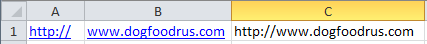
Search can be very helpful when you want to sort by keywords in a long list of domains. Domains that dont contain the keyword for which youre searching will return #VALUE whereas domains that do contain the keyword will return a number. An example might be:
=SEARCH(dog,A1)
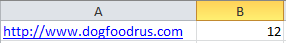
In this example, were searching for the keyword dog in a URL. This function will return the number 12 because the word dog begins at the 12th character in the URL string.
LEFT, MID, and RIGHT
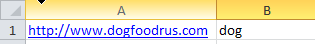
LEFT returns the leftmost characters of a string.
Example: =LEFT(A1,7) will return the leftmost seven characters in the string from cell A1.
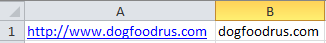
MID returns the middle characters of the string.
Example: =MID(A1,12,3) will return the characters in the string starting at position 12.
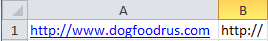
RIGHT works in a similar manner, but returns the right-most characters of the string. This can be useful for separating domain names from a domain list that contains http://www. before every domain.
Example: =RIGHT(A1,14) were returned the right-most 14 characters from the string.
These functions can be useful for pulling specified keywords, domain names, LSI data, and other information out of a string. One good example would be to copy and paste a long list of backlinks into Excel and then create a new function that searches for a specific keyword. You can then copy and paste the function down the entire column for each URL to find out how many sites use the specific keyword.
CONCATENATE
Concatenate will allow you to combine strings. This can be useful for combining pieces of a URL into one address. It can also be used to build link building queries, site maps, and keyword lists.
Example: =CONCATENATE(A1,B1) will concatenate the cells A1 and B1.
RAND
The RAND function creates a random number, which is a great way to randomly sort lists of information. Randomization is one important element of naturalness, which is the key to a successful link building campaign.
Example: placing =RAND() in every row within a column will generate a random number.
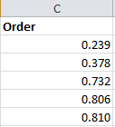
Once you have created your list of random numbers, you will then need to copy the list, and paste the values into a new column on the spreadsheet using paste as values (see image below). Paste as values is required because the random numbers will be generated each time the field is sorted. By pasting the numbers as values, you ensure the numbers wont change.
Below is an example of five URLs randomly sorted by number.
Randomly sorting lists of URLs/domains can be useful for split-testing various outreach templates while minimizing any biases that could be caused by non-randomization of the list.
OFFSET
Heres a great video tutorial of how to use the OFFSET function. According to Microsoft, offset returns a reference to a range that is a given number of rows and columns from the given reference. One example of this functions usefulness in SEO is analyzing the ranges from a Google Analytics CSV export.
Syntax: OFFSET(reference,rows,columns,[height],[width])
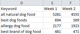
To continue with our dog food example, we start with exported data from Google Analytics (see below):
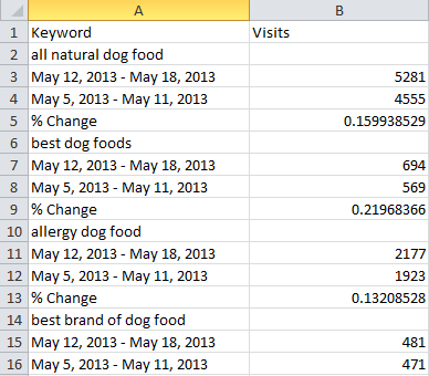
For this example, we have referring keyword traffic from one week compared to the previous week. If we were simply looking to compare a few weeks worth of data, it wouldnt be a problem. However, when you look at data like this for thousands of keywords, it can be difficult to manage.
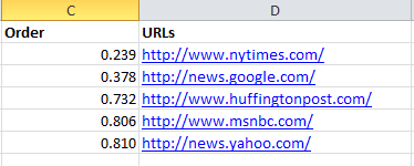
Using the OFFSET command, we can turn this list of keywords and date ranges into the following data:
Getting the first row of data is simple. Afterward, we can use the OFFSET command to grab the keyword, week 1 and week 2 data using the following formulas:
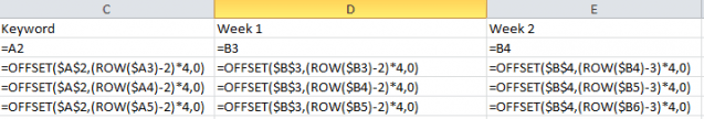
Note the ROW command returns the number of the cell where its located. This allows us to move to different rows to grab data.
INDEX and MATCH
While many Excel users like VLOOKUP, its limited in that your look up must be in the left-most column to lookup data. The INDEX command doesnt have this limitation and will return a value from a specified row and column within a given range.
Syntax: INDEX (array,row_number,[column_number])
For example, using the formula =INDEX(A1:A5,3), were able to retrieve the text from the third row of the array in column A.
MATCH adds to the power of INDEX. Unlike INDEX, which returns a word, the MATCH function returns a number.
Syntax: MATCH (value, array, [match_type])
Value is the letter or phrase that you wish to search for.
Array is the array of data that you wish to search.
Match_type specifies the type of match.
Match_type options include:
1 Less than This is the default and will find a match less than or equal to the lookup value assuming that the list is in ascending order.
-1 Greater than finds the smallest value that is greater than or equal to the lookup value assuming that the list is in descending order.
0 will return the first value that it finds that is equal to your lookup value. This is the recommended option for SEO purposes.
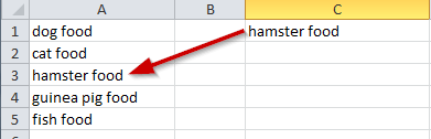
Using our pet food keyword example above, the following formula will return the location (row) in the array of the phrase guinea pig food.
=MATCH(guinea pig food,A1:A5,0)
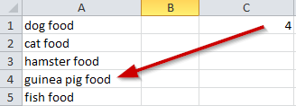
In this case, it returned the number 4 since guinea pig food is the fourth item in the list.
Combing INDEX and MATCH
You can combine INDEX and MATCH for more powerful purposes. Combine them using the following method:
=INDEX(array, MATCH formula)
Lets take, for example, our keyword list about dog food in our imaginary dogfoodrus.com website. In the table below, we have different keywords that are bringing in organic traffic for specific landing page URLs. Each row contains the number of visits and conversions associated with that keyword.
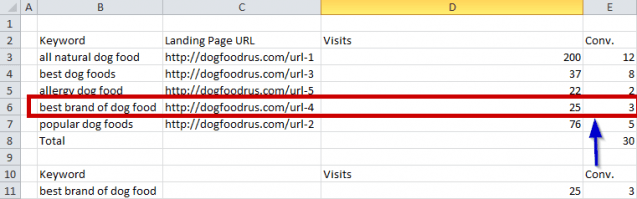
Using the INDEX and MATCH commands together, you can create a keyword lookup that will give you the number of visitors and conversions for a specific keyword. Now, if you only have four or five keywords, as in this example, looking them up manually isnt a big deal. However, if you downloaded analytics or Google Webmaster Tools data with thousands of keywords, this can be an easy way to look up specific keywords and build a specific list.
=INDEX($B$3:$E$7,MATCH(B11,$B$3:$B$7,0),3) number of visits
=INDEX($B$3:$E$7,MATCH(B11,$B$3:$B$7,0),4) number of conversions
In this example, the INDEX has a range of B3 to E7 which encompasses all of the imported data. It uses the MATCH command to specify the row within the array where the match is found. The 3 and 4 at the end of the formulas are the columns where the data you wish to copy is found.
There are many uses for INDEX and MATCH together. It can be an easy way to look up information in a huge table. Unlike VLOOKUP, INDEX and MATCH does not require the lookup field be in the leftmost column of the array.
Conclusion
These are some of the common Excel functions that I find useful when working on SEO campaigns. Excel can be used for many SEO jobs including managing backlinks, tracking keywords, visits, conversions, and much more. Do you know of any other useful Excel tips for SEO? Leave a comment and let me know!
SOURCE: http://bit.ly/17PWp8n, this factual content has not been modified from the source. This content is syndicated news that should be used for your research, and we hope that it can help your productivity. This content is strictly for educational purposes and is not made for any kind of commercial purposes of this blog.